💾 Download Notebook

import qutip as qt
import numpy as np
import matplotlib.pyplot as plt

Two-Level system

As we will be working with ions (who would have thought!) we would like to better understand their dynamics. We often consider two internal states the excited and ground states. Thus we represent ions’ degrees of freedoms as two-level systems or qubits. The Hamiltonian therefore is

where

and $\omega_{eg}$ is the energy splitting between the excited state $\vert e\rangle$ and the ground state $\vert g\rangle$. We will use the pyhton qutip package to play round with this system.

Note that, from this point onwwards, we will set $\hbar = 1$ in all the simuations.

omega_eg = 10

H_bare = 0.5*omega_eg*qt.sigmaz()
H_bare

Quantum object: dims=[[2], [2]], shape=(2, 2), type=’oper’, dtype=CSR, isherm=True\(\left(\begin{array}{cc}5 & 0\\0 & -5\end{array}\right)\)

We can conpute the discrete energy levels by computiong the eigenvalues of the Hamiltonian. Although the eigenenergies are trivial in this case, we can use qutip to compute them. In the end, we would expect an energy splitting of

Remember that the energy of the ground state is “arbitrarily” chosen, what we really care about is the splitting.

energies = H_bare.eigenenergies()
print("Energy levels:", energies)

Energy levels: [-5.  5.]

The system, as it is now, it is not that interesting. We can add a coherent drive (e.g. a laser field) that will make the dynamics of the systme more interesnting

Driven Two-Level System

If we were to start from the celebrated dipole interaction hamiltonian, expand it and perform rotating-wave approximaton (have a look at the Quantum Optics notes), we would arrive to the following interaction Hamiltonian:

where

and $\omega_L$ is the laser frequency and $\Omega$ is the Rabi frequency. Therefore, the total Hamiltonian in rotating frame becomes

where we define the detuning as $\Delta = \omega_L - \omega_{eg}$. For now, let’s assume that the detuning is zero. We get

Omega = 1*(2*np.pi)

H_int = 0.5*Omega*(qt.sigmap() + qt.sigmam())
H_int

Quantum object: dims=[[2], [2]], shape=(2, 2), type=’oper’, dtype=CSR, isherm=True\(\left(\begin{array}{cc}0 & 3.142\\3.142 & 0\end{array}\right)\)

Rabi Oscillations

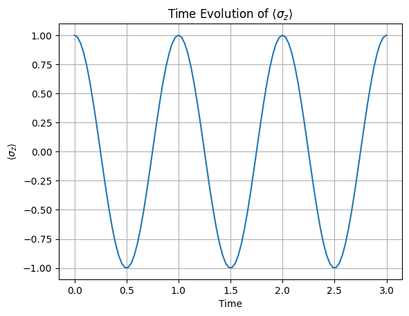
It is no secret that the resonant system will drive Rabi oscillations in the population. If we start with the excited state

we get the following time evolution:

psi_0 = qt.basis(2, 0)
psi_0

Quantum object: dims=[[2], [1]], shape=(2, 1), type=’ket’, dtype=Dense\(\left(\begin{array}{cc}1\\0\end{array}\right)\)

simulation_times = np.linspace(0, 3, 100)
solutions = qt.sesolve(H_int, psi_0, simulation_times, [qt.sigmaz()])

# Plot the results
plt.plot(simulation_times, solutions.expect[0])
plt.xlabel('Time')
plt.ylabel('$\langle\sigma_z\\rangle$')
plt.title('Time Evolution of $\langle\sigma_z\\rangle$')
plt.grid(True)
plt.show()

Introducing Dissipation

This is a good starting point! However, in the real world we will have to take into account non-idealities. In particular we will consider two sources of decoherence:

1. spontaneous emission and
2. pure decoherence

To model this phenomena we will use the Density Matrix and Lindblad Master Equation formalism. For a system subject to coherent drive $\hat{H}$, and a set of dissipative dynamics (more on that later) ${(\hat{L}_i): i = 1,2,\dots, N}$ is given by the master equation

where ${\cdot, \cdot}$ is the anticommutator. But let’s delve a bit more into the the so called Jump Operator structure. In particular $\hat{L}$ denotes the non-hermitian (or dissipative) action that the system is subject to, and is usually expressed as

Therefore, $\hat{O}$ represents the action of the jump operator, while $\gamma_i$ gives its strenght.

Spontaneous Emission

As you will know, the coupling of the atom to the continuum of electromagentic field modes will cause spontaneous emission to occurr. The jump operator therefore becomes

We can implement it in qutip as follows. As an initial example, let’s consider the bare system being initialised in its excited state. We will expect an exponential decay of the excited population from the spontaneous decay:

rho_0 = psi_0 * psi_0.dag()
rho_0

Quantum object: dims=[[2], [2]], shape=(2, 2), type=’oper’, dtype=Dense, isherm=True\(\left(\begin{array}{cc}1 & 0\\0 & 0\end{array}\right)\)

decay_rate = 3
L_se = np.sqrt(decay_rate)*qt.sigmam()
L_se

Quantum object: dims=[[2], [2]], shape=(2, 2), type=’oper’, dtype=CSR, isherm=False\(\left(\begin{array}{cc}0 & 0\\1.732 & 0\end{array}\right)\)

solutions_se = qt.mesolve(H_bare, rho_0, simulation_times, [L_se], [qt.sigmaz()])

# Plot the results
plt.plot(simulation_times, solutions_se.expect[0], 'green')
plt.xlabel('Time')
plt.ylabel('$\langle\sigma_z\\rangle$')
plt.title('Time Evolution of $\langle\sigma_z\\rangle$')
plt.grid(True)
plt.show()

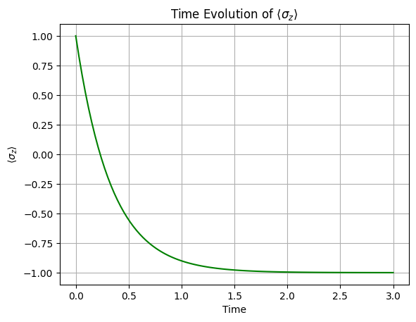
Great, this is ax expected: as time passes by a photon is more lilely to be emitted and the atom decays to the ground state. Let’s go back to the driven state and see what happnes:

solutions_se_int = qt.mesolve(H_int, rho_0, simulation_times, [L_se], [qt.sigmaz()], options={'store_states': True})
# Plot the results
plt.plot(simulation_times, solutions.expect[0])
plt.plot(simulation_times, solutions_se_int.expect[0])
plt.xlabel('Time')
plt.ylabel('$\langle\sigma_z\\rangle$')
plt.title('Time Evolution of $\langle\sigma_z\\rangle$')
plt.grid(True)
plt.show()

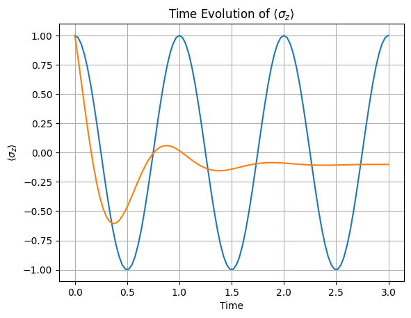
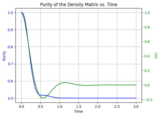
We see that as time passes, the rabi oscillations are damped. This is because the spontaneous emission causes decoherence to decay. Once the state is in a mixed state, all contrast is gone as the coherence is lost. We can in fact plot the purity of the state as a function of time.

purity_values = [rho.purity() for rho in solutions_se_int.states]

fig, ax1 = plt.subplots()
ax1.plot(simulation_times, purity_values, color='blue')
ax1.set_xlabel('Time')
ax1.set_ylabel('Purity', color='blue')
ax1.tick_params(axis='y', labelcolor='blue')

ax2 = ax1.twinx()
ax2.plot(simulation_times, solutions_se_int.expect[0], color='green')
ax2.set_ylabel('$\langle\sigma_z\\rangle$', color='green')
ax2.tick_params(axis='y', labelcolor='green')

plt.title('Purity of the Density Matrix vs. Time')
ax1.grid(True)

plt.show()

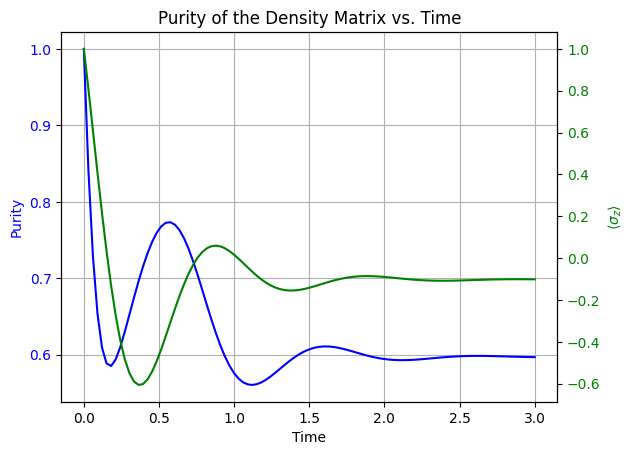
What is interesting is that the spontaneous emission is in the end driving us towards a pure state, or the ground state!

Pure Decoherence

We consider another source of decoherence. In this case we do not modify the energy of the state (as we saw in spontaneous decay, as we emitted a photon). In the lab, pure decoherence might come from a laser’s intensity noise, that will make the Rabi frequency fluctuate. The corresponding jump operator is

depahsing_rate = 3
L_d = np.sqrt(depahsing_rate)*qt.sigmaz()
L_d

Quantum object: dims=[[2], [2]], shape=(2, 2), type=’oper’, dtype=CSR, isherm=True\(\left(\begin{array}{cc}1.732 & 0\\0 & -1.732\end{array}\right)\)

solutions_se_d = qt.mesolve(H_bare, rho_0, simulation_times, [L_d], [qt.sigmaz()])

# Plot the results
plt.plot(simulation_times, solutions_se_d.expect[0], 'green')
plt.xlabel('Time')
plt.ylabel('$\langle\sigma_z\\rangle$')
plt.title('Time Evolution of $\langle\sigma_z\\rangle$')
plt.grid(True)
plt.show()

As expected, in this case we do not decay from the excited state to the ground state. Let’s now have a look at the driven system

solutions_d_int = qt.mesolve(H_int, rho_0, simulation_times, [L_d], [qt.sigmaz()], options={'store_states': True})
purity_values = [rho.purity() for rho in solutions_d_int.states]

fig, ax1 = plt.subplots()
ax1.plot(simulation_times, purity_values, color='blue')
ax1.set_xlabel('Time')
ax1.set_ylabel('Purity', color='blue')
ax1.tick_params(axis='y', labelcolor='blue')

ax2 = ax1.twinx()
ax2.plot(simulation_times, solutions_d_int.expect[0], color='green')
ax2.set_ylabel('$\langle\sigma_z\\rangle$', color='green')
ax2.tick_params(axis='y', labelcolor='green')

plt.title('Purity of the Density Matrix vs. Time')
ax1.grid(True)

plt.show()