1. Manipulating Qubits
Today we will briefly go over the basics of quantum mechanics and quantum information processing from the algorithmic perspective.
Quantum Mechanics Crash Course
The natural quantum extension of the bit to the quantum world is the qubit. Classically a bit can have only two values $0$ or $1$. In quantum mechanics, we represent qubit states with vectors, namely
\[|0\rangle = \begin{pmatrix} 1 \\ 0 \end{pmatrix} \ \text{and} \ |1\rangle = \begin{pmatrix} 0 \\ 1 \end{pmatrix}\]| Therefore, a qubit can be $ | 0\rangle$, $ | 1\rangle$ or a coherent superposition of the two poissible states, namely: |
We can extend to the concept of multiple qubits via the tnesor product operator $\otimes$. The composite state of a multi-qubit system is iven by the tensor product of the states of its constituents. For example if we have the two qubit states
\[|\psi_A\rangle = a_A|0_A\rangle + b_A |1_A\rangle \\ |\psi_B\rangle = a_B|0_B\rangle + b_B |1_B\rangle\]| The two qubit state $ | \Psi\rangle$ becomes |
where we dropped the indexes for the different qubits and removed the explicit tensor product operator. Underlying vectors compose according to… you guessed it, the tensor product operrator. For example
\[|00\rangle = \begin{pmatrix} 1 \\ 0 \end{pmatrix} \otimes \begin{pmatrix} 1 \\ 0 \end{pmatrix} = \begin{pmatrix} 1 \times \begin{pmatrix} 1 \\ 0 \end{pmatrix}\\ 0 \times \begin{pmatrix} 1 \\ 0 \end{pmatrix} \end{pmatrix} = \begin{pmatrix} 1 \\ 0 \\ 0 \\ 0 \end{pmatrix}\]We already notice an interesting scaling here. To represent (save) $N$ bits of classical information we will require $N$ bits. Namely, if you want to write down $N$ bits… well, there they are. Conversely, if we have $N$ qubits, we will roughly need $2^N$ pieces of information that we need to keep track off. Think about the case for $N = 2$ (as written above). Broadly speaking, to specify any given state of a tqo-qubit system we will need to write down four numbers $A, B, C$ and $D$. You will get back to this on the problem sheet.
Operations on Qubits
If states are represented by vectors, operators are represented by matrices. It turns out that such matrices need to be hermitian to represent physical observables. This is strictly related to the unitarity of the SE.
Hermitian operators on qubits (or two-level systems) can be written in terms of the pauli operators. You better memorise them!
\[\sigma_x = \begin{pmatrix} 0 & 1 \\ 1 & 0 \end{pmatrix}, \ \sigma_y = \begin{pmatrix} 0 & -i \\ i & 0 \end{pmatrix}, \ \sigma_z = \begin{pmatrix} 1 & 0 \\ 0 & -1 \end{pmatrix}, \ \mathbb{I} = \begin{pmatrix} 1 & 0 \\ 0 & 1 \end{pmatrix}\]By construction, any hermitian operator can be written as a linear superposition of pauli matrices, namely
\(H = \alpha \mathbf{I} + \vec{r} \cdot\vec{\sigma}\) where $\vec{\sigma} = [\sigma_x, \sigma_y, \sigma_x]^T$. Therefore, it makes sense to study the properties of pauli matrices. Something important (and useful) to remember is that \(\sigma_x^2 = \sigma_y^2 = \sigma_z^2 = \mathbb{I} \\ [\sigma_x, \sigma_y] = 2i\sigma_x \ \text{and rotations}\)
| For any observable (operator) $\hat{O}$, and given a state $ | \psi\rangle$, the expecation value of the observable is given by |
where $\langle\psi\vert$ is the dual of $\vert\psi\rangle$, namely its hermitian conjugate. For example
\[\langle\psi| = \begin{pmatrix} 1 \\ 0 \end{pmatrix}^\dagger = \begin{pmatrix} 1 & 0 \end{pmatrix}\]The variance can be calculated as usual
\[\text{Var}_{|\psi\rangle}\{\hat{O}\} = \langle \hat{O}^2 \rangle_{|\psi\rangle} - \langle \hat{O} \rangle^2_{|\psi\rangle}\]Bloch Sphere Representation
Let us go back to the state of a single qubit, recall from above that we have
\[|\psi\rangle = a|0\rangle + b |1\rangle\]subject to the constraint
\[|a|^2 + |b|^2 = 1\]Looking at the constraint, we can write both $a$ and $b$ in terms of sine and cosine, as well as a complex phase, namely
\[a = \cos\left(\frac{\theta}{2}\right) e^{i\phi_1} \\ b = \sin\left(\frac{\theta}{2}\right) e^{i\phi_2}\]We note that this satify the constraint above, thus we rewrite the qubit state as
\[|\psi\rangle = \cos\left(\frac{\theta}{2}\right) e^{i\phi_1}|0\rangle + \sin\left(\frac{\theta}{2}\right) e^{i\phi_2} |1\rangle\]Since quantum states are quivalent up to a global phase, we can collect $e^{i\phi_1}$ and define $\phi = \phi_2 - \phi_1$ to get to
\[|\psi\rangle = \cos\left(\frac{\theta}{2}\right)|0\rangle + e^{i\phi}\sin\left(\frac{\theta}{2}\right) |1\rangle\]Due to the normalisation, we are left with two parameters, that conveniently describe the surface of a sphere (spherical coordinate system). The factor of $1/2$ in $\theta$ will become apparent later. It is sufficient to say that for any pair of $(\theta, \phi)$ we can associate a point on a sphere.
Pauli Operators as Rotations
From the Schrodinger equation we get the time propagator opearator as
\[U(t) = e^{-\frac{i H t}{\hbar}}\]We can now chose the Hamiltonian $H$ to be of the form
\[H = \hbar \, \vec{\sigma} \cdot \vec{n}\]Where $\vec{n}$ is a normal vector, we can therefore plug it into the time propagator and we get
\[U(t) = e^{-i \, \vec{\sigma} \cdot \vec{n} t }\]We can chose $t = \theta/2$, and we get the following:
\[R_{\vec{n}}(\theta) = e^{-i \frac{\theta}{2} \vec{\sigma} \cdot \vec{n}}\]Making use of the properties of pauli matrices, we can rewrite it in the form
\[R_{\vec{n}}(\theta) = \cos\left(\frac{\theta}{2}\right)\mathbf{I} - i \sin\left(\frac{\theta}{2}\right) (\vec{\sigma} \cdot \vec{n})\]You can compute its action on a generic qubit state, to confirm that the action of $R$ is to rotate the state around the vector $\vec{n}$ by an angle $\theta$.
QIP I Crash Course
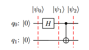
We will now briefly talk about two gates. The single qubit gate $H$ (or Hadamard gate) and the two-qubit gage $CNOT$.
The Hadamard Gate
The Hadamard gate takes maps the states $|0\rangle$ and $|1\rangle$ to $|+\rangle$ and $|-\rangle$ respectively, where
\[|\pm\rangle = \frac{1}{\sqrt{2}}(|0\rangle \pm |1\rangle)\]We can write the action of the Hadamard gate in terms of the Pauli gates $X, Y, Z$. Such operators, rotate the state about each respective axis by $\pi$ radians. You can easily check that the Hadamard gate, has the following form
\[H = \frac{1}{\sqrt{2}}(X + Z)\]Therefore its matrix representation becomes
\[H = \frac{1}{\sqrt{2}} \begin{pmatrix} 1 & 1 \\ 1 & -1 \end{pmatrix}\]You can easily check that the action of the $H$ gate is as described aboove. We usually avoid having to write the gates’ matrix expression. Instead we work with circuit diagrams. Each qubit is an horizontal line and gates are expressed as blocks.