11. An Intro to Quantum Error Correction
In the previous sections, we have seen how we can build quantum processing units using different architecture. While each architecture has its own advantages and disadvantages, all physical implementations of quantum computers suffer from decoherence. For instance, phase fluctuations in lasers lead to decoherence in neutral and trapped ion systems. Although we can think of making our systems better and better, by throwing money and engineering at the problem, we need to make quantum information itself more robust. This is where quantum error correction (QEC) comes into place.
Similar challenges are enountered by computer scientists and information theorists. While the physical error rates of classical information processing (i.e. CPUs) is much lower than for QIP, classical communication channels are notoriously noisy. Think of the static that AM/FM radio exhibits. Thus classical error correction played (and still plays) a bit role in digital communication systems.
We will develop the core idea of error correction by considering classical systems, to the move to the stavbilizer formalism used in QEC.
Making Information Redundant
Alice wants to send a bit string $s_i \in {0,1}$, with $i=1,\dots,N$. On the other side, Bob receives the message that Alice has sent, but he might misinterpret what he is receiving because of some interference. For example the bit string gets misinterpreted as
\[001011 \to 000011\]We noticed that a bit flip has happened on the $i=3$ (third) bit. What is problematic here is that Bob has no way of telling that an error has occurred, let alone correcting it. This is because both the errorless $001011$ and the misinterpreted $000011$ bit strings are valid. A possible solution is to make information redundant, in a way that allows us to detect (and possibly correct errors). To achieve this, we assign to each logical bit (i.e. the bit that Alice wants to send) a codeword. For instance
\[\tilde{0} \to 000 \\ \tilde{1} \to 111\]where the tildes indicate logical bits. We see that our code space (the space consisting of all the codewords) consists of a repetition of our logical qubit. Therefore, Alice’s original message would become
\[000,000,111,000,111,111\]where we have added commas for ease of reading. If an error would still happen on the third physical bit (the actual bits that are being sent), Bob would receive the following message
\[001,000,111,000,111,111\]But now Bob has the way of detecting that an error has occurred. In fact, the first word is not part of the original code space. Therefore Bob concludes that an error must have occurred. We can push this idea one step further and ask ourselves what is the most likely error to have occurred. If we (reasonably) assume that only single bit-flip errors occur, then we conclude that $001$ must be mapped to $000$. Thus, simply by repeating information and looking at the majority of the bits in a word, we are able to detect and correct classical errors. This is called the Repetition Code.
Note the it is possible to fool ourselves. For instance, if we were unlucky enough to have 2 bit flips per word, for instance
\[\tilde{0} = 000 \to 011,\]we would still be able to detect that an error has occurred, but if we were to correct it, we would correct it to the wrong logical bit $\tilde{1}$. Even worse, if three errors were to occur,
\[\tilde{0} = 000 \to 111 = \tilde{1},\]we would not even be able to detect that an error occurred, leaving us completely in the dark. This can be mitigated with better error correcting codes at the expense of having to send more information. For instance one could use the code space mapping to be
\[\tilde{0} \to 0000 \\ \tilde{1} \to 1111\]Going Quantum
It turns out that classical error correction codes can be readily transposed to quantum alorithms, except for one big problem. When considering the repetition code, detecting and correcting errors involved looking at the state of each bit. Now we can simply map each logical qubit to a repetition of three physical ones (like in the classical counterpart), namely
\[\vert\tilde{0}\rangle \to \vert000\rangle \\ \vert\tilde{1}\rangle \to \vert111\rangle\]Like before, we can try to send a qubit from Alice to Bob, let’s pick $\vert\tilde{0}\rangle$. If a bit flip were to happen, Bob would still be able to correct for it!
\[\vert000\rangle \to \vert001\rangle\]In fact, Bob could measure the state of the three qubits and revert it back inot the correct code word. And here is the problem, Bob had to measure the state of the qubits. In this case, this was not problematic as we were dealing with eigenstates of the measurement basis (and measuring had no effect on the state). However, what if we wanted to send the more general state
\[\vert\tilde{\psi}\rangle = \frac{\vert\tilde0\rangle+\vert\tilde1\rangle}{\sqrt{2}}\]In this case, if a bit flip were to occur on the third bit, we would get
\[\frac{\vert000\rangle+\vert111\rangle}{\sqrt{2}} \to \frac{\vert001\rangle+\vert110\rangle}{\sqrt{2}}\]When Bob tries to measure the state, he would collapse the state into either $\vert001\rangle$ or $\vert110\rangle$, thus destroying it. Therefore, we need a more clever way of detecting (and correcting) errors. In particular, we want to find a way to
- Measure the error that occurred only.
- Leave the underlying state untouched.
This can be formalised in the stabiliser formalism
The Stabiliser Formalism
Consider a code space $\mathcal{C}$, such that any logical qubit $\vert\tilde\psi\rangle \in \mathcal{C}$. In the case of the simple three-qubit repetition code $\mathcal{C} = \text{span}{\vert000\rangle, \vert111\rangle}$. Now, the stabiliser group $\mathbb{S}$ is defined as follows
\[\mathbb{S} = \left\{S \in \mathbb{G} \ \Big\vert\ S \vert\tilde\psi\rangle = \vert\tilde\psi\rangle \quad \forall\vert\tilde\psi\rangle \in C\right\}\]where $\mathbb{G}$ is the Pauli group for $n$ qubits. In other words, a stabiliser $S$ is any composition of Pauli operators (e.g. $X_1Y_2\mathbb{I}_3$) that leaves all states within the codesapce $\mathcal{C}$ untouched. Then, the group $\mathbb{S}$, holds all the possible stabilisers. Now, considering our three-qubit reperition code, the stabiliser group would be
\[\mathbb{S} = \left\{Z_1Z_2, Z_1Z_3, Z_2Z_3\right\}\]To detect (and correct) errors, we then apply the stabilisers to our code words and measure the result.
| State | $Z_1Z_2$ | $Z_1Z_3$ | $Z_2Z_3$ | Error Type |
|---|---|---|---|---|
| $\vert000\rangle, \vert111\rangle$ | +1 | +1 | +1 | No Error |
| $\vert100\rangle, \vert011\rangle$ | -1 | -1 | +1 | Bit Flip on 1st qubit |
| $\vert010\rangle, \vert101\rangle$ | -1 | +1 | -1 | Bit Flip on 2nd qubit |
| $\vert001\rangle, \vert110\rangle$ | +1 | -1 | -1 | Bit Flip on 3rd qubit |
We see that just by looking at the results of the three stabilisers, we can detect what type of error happened, and eventually correct for it. Most importantly, this is done without collapsing the loical state. Additionally, if we look closely, we only need to measure $Z_1Z_2$ and $Z_2Z_3$, since the information in $Z_1Z_3$ is redundant. Therefore, to perform error correction we can
- Perform the stabilisers check. This is done by a series of $CNOT$ gates structured according to the stabilisers. The outcome is then “stored” and read from ancilla qubits
- Decode the error from the syndrome (result of the stabiliser checks) and apply a conditional unitary transformation to correct for the error
In the case of our simple three-qubi repetion code, we can use the circuit below.
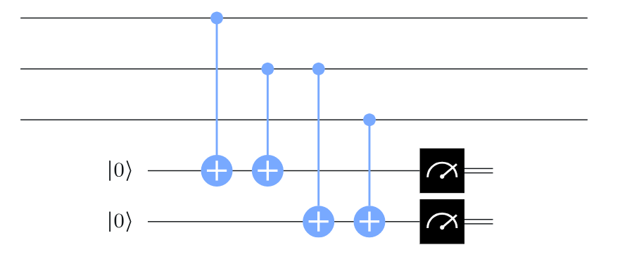
Image reproduced from (https://quantum.cloud.ibm.com/learning/en/courses/foundations-of-quantum-error-correction/correcting-quantum-errors/repetition-codes)
Notice the three qubit on the top used to store the code word and the bottom two ancilla qubits. The top ancilla holds the $Z_1Z_2$ stabiliser check information, while the bottom ancilla holds the $Z_2Z_3$ stabiliser check information.
It is then possible to decode the information to correct for the error according to
| $Z_1Z_2$ | $Z2Z_3$ | Action |
|---|---|---|
| +1 | +1 | $\mathbb{I}$ (do nothing) |
| -1 | +1 | $X_1$ (flip 1st bit) |
| -1 | -1 | $X_2$ (flip 2nd bit) |
| +1 | -1 | $X_3$ (flip 3rd bit) |
Analogue Errors
Up until now we have consider only “digital” quantum errors. However, we can consider errors that go beyond bit flips. For example, we might have a linear combination of errors. In the most general case, we would have
\[\vert000\rangle \to \alpha\vert000\rangle + \beta\vert100\rangle + \gamma\vert010\rangle + \delta \vert001\rangle\]What would happen if we were to perform the stabiliser check? Well we would collapse this superposition of errors into a single error, with the associated probability. This is because, by measuring the syndrome, we are effectively measuring the error. Thus, like any other quantum state, when measuring the error we collapse it into one of its eigenstates. This can be summarised in the following table
| $Z_1Z_2$ | $Z2Z_3$ | State After Stabilizer Check | Probability | Action |
|---|---|---|---|---|
| +1 | +1 | $\vert000\rangle$ | $|\alpha|^2$ | $\mathbb{I}$ (do nothing) |
| -1 | +1 | $\vert100\rangle$ | $|\beta|^2$ | $X_1$ (flip 1st bit) |
| -1 | -1 | $\vert010\rangle$ | $|\gamma|^2$ | $X_2$ (flip 2nd bit) |
| +1 | -1 | $\vert001\rangle$ | $|\delta|^2$ | $X_3$ (flip 3rd bit) |
Beyond $X$-Like Errors
Before concluding, it is important to note that compared with classical methods, quantum error correction schemes need to take into account an extra type of error. While we have only considered bit flips (or $X$) errors, a good quantum error correction scheme needs to take into accound als phase (or $Z$) errors. Since $ZX = iY$, this is sufficient to correct for any Pauli error. An example of such code, is The 9-Qubit Shor Code.