2. Atoms (Ions) as Qubits
We have seen how we describe the state of a qubit on the Bloch Sphere. In addition, we have seen that we can apply gates to our qubit to manipulate its state. However, in practice, how do we implement a gate?
Atom-Light Interaction
Consider the electronic structure of an atom (ion). Here, we will consider $^{40}\text{Ca}^+$ electronic structure.
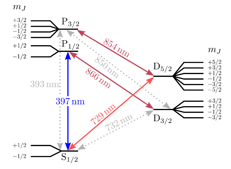
Image reproduced from R. Oswald, Characterization and control of a cryogenic ion trap apparatus and laser systems for quantum computing
To build a qubit, we can (wisely) select any two levels and call them the ground $\vert0\rangle$ and excited $\vert1\rangle$ states accordingly. We will neglect all the other states, and the model of our atom’s internal degree of freedom becomes of a qubit. We assume that the energy levels are split by $\omega_{eg}$, thus the hamiltonian becomes
\[H = \frac{\hbar\omega_{eg}}{2}\vert1\rangle\langle 1\vert - \frac{\hbar\omega_{eg}}{2}\vert0\rangle\langle 0\vert = \frac{\hbar\omega_{eg}}{2}\sigma_z.\]We immediately see that both $\vert 0\rangle$ and $\vert 1\rangle$ are eigenstates of this Hamiltonian. To manipulate the state, we need to interact with the ion. You will need to trust me (or take quantum optics), to see that the Hamiltonain for a dipole-allowed transition subject to an Electric field becomes
\[H = \frac{\hbar\omega_{eg}}{2}\sigma_z - \mathbf{d} \, \cdot \, \mathbf{E}(t),\]where $\mathbf{d}$ is the dipole operator coupling the ground and excited states and $\mathbf{E}(t)$ is a time-varying applied electric field. You will have to, once again, trust me (or take atomi physics) to see that the form of the dipole operator is
\[\mathbf{d} = \vec{\mu}\left(|1\rangle\langle 0| + |0\rangle\langle 1|\right) = \vec{\mu}(\sigma_+ + \sigma_-)\]where $\vec{\mu}$ is a vector constant (dipole moment) set by the transition. The form of the electric field is given by
\[\mathbf{E}(t) = \vec{E}_0e^{-i\omega t} + \vec{E}_0^*e^{i\omega t}\]where $\phi$ is the phase of the light field. We can now substitute and get
\[\mathbf{d} \, \cdot \, \mathbf{E}(t) = \vec{\mu} (\vec{E}_0e^{-i\omega t} + \vec{E}_0^*e^{i\omega t})(\sigma_+ + \sigma_-)\]where the Rabi frequency $\Omega$ indicates the coupling strength of the oscillating electric field with the electronic transition. We will now move to the intraction picture via the unitary transform
\[H \to UHU^\dagger + i\hbar\dot{U}U^\dagger.\]We assume that the laser field is on resonance with the transition $\omega = \omega_{eg}$, therefore we choose
\[U = e^{\frac{i\omega\sigma_z}{2}t}\]We see that the second term becomes
\[i\hbar\dot{U}U^\dagger = -\frac{\hbar\omega}{2}\sigma_z\]thus cancelling the first term on the Hamiltonian. To better compute the second term, we compute
\[e^{\frac{i\omega}{2}\sigma_zt}\sigma_{\pm}e^{-\frac{i\omega}{2}\sigma_zt} = e^{\pm i\omega t}\sigma_\pm\]If we substitute back in, we get that the Hamiltonian in interaction picture
\[H_I = -\vec{\mu}(\vec{E}_0\,\sigma_+\,e^{i\omega t}e^{-i\omega t} + \vec{E}_0\,\sigma_-\,e^{-i\omega t}e^{-i\omega t} + \text{h.c})\]We now drop the fast oscillating terms at $2\omega$ and we are left with the following
\[H_I = -\vec{\mu}(\vec{E}_0\sigma_+ + \vec{E}_0^*\sigma_-)\]We now write the electric field as
\[\vec{E}_0 = \vec{n} \, E_0 e^{i\phi}\]and the expression above becomes
\[H_I = -E_0(\vec{\mu}\cdot\vec{n})(e^{i\phi}\sigma_+ + e^{-i\phi}\sigma_-)\]We can now substitute the expressions
\[\sigma_{\pm} = \sigma_x \pm i\sigma_y\]and we get that
\[\begin{align*} H_I &= \frac{\hbar\Omega}{4}(e^{i\phi}\sigma_x + ie^{i\phi}\sigma_y + e^{-i\phi}\sigma_x -ie^{-i\phi}\sigma_y) \\ &= \frac{\hbar\Omega}{2}\left(\frac{e^{i\phi} + e^{-i\phi}}{2}\,\sigma_x - \frac{e^{i\phi} - e^{-i\phi}}{2i}\,\sigma_y\right) \\ &= \frac{\hbar\Omega}{2}(\cos\phi \,\sigma_x - \sin\phi\,\sigma_y) \end{align*}\]We can see that we can tune wether we get a $X$ or $Y$ interaction by tuning the phase $\phi$ of the incident field.
Driving Gate Operations
We now see how we can use a $\sigma_x, \sigma_y$ type of Hamiltonian to implement our beloved gates. To this end, we need to start from the Schrodinger equation.
\[i\hbar \frac{\partial}{\partial t} \ket{\psi(t)} = \hat{H}(t)\ket{\psi(t)}\]To solve for the time dynamics, we can rearrange and integrate both sides
\[\begin{align*} \frac{\mathrm{d}\ket{\psi(t)}}{\ket{\psi(t)}} &= -\frac{i}{\hbar} \hat{H}(t)\,\mathrm{d}t \\ \int_{\ket{\psi(0)}}^{\ket{\psi(\tau)}} \frac{\mathrm{d}\ket{\psi(t)}}{\ket{\psi(t)}} &= -\frac{i}{\hbar} \int_{0}^{\tau} \hat{H}(t)\,\mathrm{d}t \\ \ket{\psi(\tau)} &= e^{-\frac{i}{\hbar} \int_{0}^{\tau} \hat{H}(t)\,\mathrm{d}t}\ket{\psi(0)}. \end{align*}\]By substituting $\tau \to t$ and $t \to t^\prime$ in the expression above we get
\[\begin{equation} \ket{\psi(t)} = \underbrace{\exp\left(-\frac{i}{\hbar} \int_{0}^{t} \hat{H}(t^\prime)\,\mathrm{d}t^\prime\right)}_{U(t)}\ket{\psi(0)}. \end{equation}\]For a time-independent Hamiltonian, the time propagator reduces to
\[U(t) = \exp\left(-i\hat{H}t/\hbar\right)\]Now assume we drive a $\sigma_x$ type of interaction, namely
\[H = \frac{\hbar\Omega}{2}\sigma_x\]We can substitute in the expression above, to get the following
\[U(t) = \exp\left(-i\frac{\theta}{2}\sigma_x\right)\]where $\theta = \Omega t$. Let’s chose $t$ such that $\theta = \pi$. We can then rewrite $U$ as
\[U = \cos\left(-\frac{\pi}{2}\right)\mathbb{I} + i \sin\left(-\frac{\pi}{2}\right)\sigma_x\]neglecting any global phase, we get that
\[U = \sigma_x\]Therefore, we see that we have implemented a $\sigma_x$ gate.