3. Atomic Physics and Dynamical Decoupling
We will explore atomic structures and how they are used as qubits.
Spectroscopic Notation
We start from the electronic configuration of $\text{Ca}$, that is given by $\text{[Ar]}\,4s^2$. If we remove one electron (since I like ions more than atoms), we are left with a single electron in the outer shell, namely $\text{[Ar]}\,4s^1$.
We now want to consider the total electron angular momentum
\[J = L + S\]For this electron we have that $L = 0$ since it is in an $s$-orbital and $S = 1/2$. From the addition rules of angular momentum we get
\[J = \frac{1}{2}\]We can enclose all this information into a single piece of information, namely
\[n^{2s + 1}L_J\]In this case we get $4^2S_{1/2}$. We can continue and think about the electron being excited into the $P$ orbital. In this case we have $L = 1/2$, $S = 1$. Therefore we would get out two statemanifolds, namely
\[4^2P_{1/2} \ \text{and} \ 4^2P_{3/2}\]Similarly, considering the $D$-orbital ($L = 2$) we get
\[4^2D_{3/2} \ \text{and} \ 4^2D_{5/2}\]We can write the state diagram as
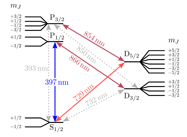
Image reproduced from R. Oswald, Characterization and control of a cryogenic ion trap apparatus and laser systems for quantum computing
The Hyperfine Structure
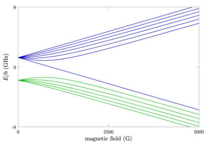
Let’s now go one step deeper. Let’s consider one additional degree of freedom, the nuclear spin $I$. This gives rise to the hyperfine structure. Consider the $5^2S_{1/2}$ level of $^{85}\text{Rb}$, experimentally we can measure its energy levels
We see that the levels are further split. To undertand what is going on here, we need to have a look at the hamiltonian
\[H = \underbrace{A\,\mathbf{I}\cdot\mathbf{J} }_\text{hyperfine interaction}+ \underbrace{\mu_B\, ( g_J\, \mathbf{J} + g_I\, \mathbf{I} ) \cdot \mathbf{B}}_\text{Zeeman interaction}\]When $B$ is small we can try to interpret the results as follows. Consider the total angular momentum
\[F = I + J\]If we now consider
\[F^2 = I^2 + J^2 + 2I\cdot J\]Therefore the hyperfine interaction term becomes
\[H_\text{HF} = \frac{A}{2}(F^2 - I^2 - J^2)\]In this case, for $B = 0$, we will have two possible values of $F$:
\[F = I \pm \frac{1}{2}\]As we start to crank up the magnetic field $B$, we will need to apply corrections to the energy levels in terms of perturbations. Here we see all the energy levels.
Let’s try to reason, what is $I$?
Repumping
We talked about how we want to prepare a qubit in a definite state. Let us consider calcium again. We define our qubit between the $S_{1/2}$ and the $D_{5/2}$ manifolds. Specifically in the $m_J = -1/2$ levels.
Assume that the population is initially randomly distributed between those two levels, how can we drive the population into the ground state?
Can we use unitary evolution here? If not, what is the problem?
The solution is that we need an additional state. In this case the $P_{3/2}$. We can drive coherent evolutions into that, which will now decay out of the $P$-manifold, back to the ground state. But which ground state? We need to repump out of the other state to then decay back.
Dynamical Decoupling
We now discuss a mathod to mitigate the effect of noise on the time-evolution of the qubit state. To this end, let’s us consider a two-level system initially in the state
\[|\psi(0)\rangle = \frac{1}{\sqrt{2}}(|0\rangle + |1\rangle)\]The atom-only Hamiltonian is given by
\[H = \frac{\hbar\omega_{eg}}{2}|1\rangle\langle 1| - \frac{\hbar\omega_{eg}}{2}|0\rangle\langle 0| = \frac{\hbar\omega_{eg}}{2}\sigma_z.\]And the associated time propagator is given by
\[U(t) = \exp\left(\frac{i\omega t}{2}\sigma_z\right)\]Therefore, the time-evolved state is given by
\[|\psi(t)\rangle = \frac{1}{\sqrt{2}}\exp\left(\frac{i\omega t}{2}\sigma_z\right)(|0\rangle + |1\rangle)\]Since both $\vert0\rangle$ and $\vert1\rangle$ are eigenstates of $\sigma_z$ with eigenvalues $-1$ and $+1$ respectively, the expression for the time-evolved state becomes
\[\begin{align*} |\psi(t)\rangle &= \frac{1}{\sqrt{2}}(e^{-\frac{i\omega t}{2}}|0\rangle + e^{+\frac{i\omega t}{2}}|1\rangle) \\ &= \frac{1}{\sqrt{2}}(|0\rangle + e^{i\omega t}|1\rangle) \end{align*}\]We see that the effect of this Hamiltonian is to rotate the state vector on the equator of the Bloch sphere. Now assume that the evolution frequency is subject to some sort of error, namely
\[\omega \to \omega + \delta\omega(t),\]where $\delta\omega(t)$ is a tim varying noise term. We can assume that $\delta\omega(t)$ evolves much slower compared to an experiment sequence, effectively yielding to a value that is randomly sampled from some distribution, namely
\[\delta\omega \sim \mathcal{N}(0, \sigma)\]Therefore, if we were to let the state evolve over time, we would accumulate a phase uncertainty
\[\delta\theta = \delta\omega \cdot t\]We can get around this with dynamical decoupling. The idea is to let the system evolve for $t/2$, then apply a $X$ gate. Let’s see what happens. Our initial state is
\[|\psi(0)\rangle = \frac{1}{\sqrt{2}}(|0\rangle + |1\rangle)\]After $t/2$ the state becomes
\[|\psi_-(t/2)\rangle = \frac{1}{\sqrt{2}}(|0\rangle + e^{i\frac{\delta\theta}{2}}|1\rangle)\]We then apply the $X$ gate and get
\[|\psi_+(t/2)\rangle = \frac{1}{\sqrt{2}}(|1\rangle + e^{i\frac{\delta\theta}{2}}|0\rangle)\]note that we flipped both bits. We now let evolve for another $t/2$ to get
\[\begin{align*} |\psi(t)\rangle &= \frac{1}{\sqrt{2}}(e^{i\frac{\delta\theta}{2}}|1\rangle + e^{i\frac{\delta\theta}{2}}|0\rangle) \\ &= \frac{1}{\sqrt{2}}(|0\rangle + |1\rangle) \end{align*}\]Here we completely removed the effect of any slow drift. By design, the echo pulses would accentuate any signal at the echo period.