5. Laser Cooling and Trapping
This set of notes is heavily inspired from Jonathan Home’s course on Quantum Optics.
If we want to use atoms (either neutral or ions) as qubits, we need to first confine them. To achieve this we will need
- a confining potential and
- a way to remove energy (cool) fast (hot) atoms
In this session, we will explore both.
The Force on an Atom
We consider a laser shining onto an atom. As we will see, the imparted light will exert a force (or a pressure) on the atom. This will be the basis mechanism that we will use to cool and trap atoms
We begin by considering, once again, a single atom coupled to the electric field of a laser. We have seen that, in the dipole approximation, the Hamiltonian of this system in the Schrodinger (lab-frame picture) is given by
\[H = \frac{\hbar\omega_{eg}}{2}\sigma_z + \frac{\mathbf{\hat{P}}^2}{2m} + \mathbf{d} \, \cdot \, \mathbf{E}(t, \mathbf{r}),\]where $\mathbf{r}$ is the position of the atom. Note that this time we are also considering the kinetic energy of the atom, since we are interested in its motion. Similarly to what we have done before, we can explicitly write the electric field as
\[\mathbf{E}(t, \mathbf{r}) = f(\mathbf{r})\cdot\mathbf{E}_0\left(e^{i(\mathbf{k}\cdot\mathbf{r}-\omega t)} + e^{-i(\mathbf{k}\cdot\mathbf{r}-\omega t)}\right).\]Once again, note that we are now also wirting the spatial terms, as ultimately we want to study the motion of the ion. Also note that we introduced a function $f$ that modulates the amplitude of the laser field depending on the position. This function’s use will become apparent later. If we plug in the expression for the elecric field into the system Hamiltonian, and expand the dipole operator $\mathbf{d}$ we get
\[H = \frac{\hbar\omega_{eg}}{2}\sigma_z + \frac{\mathbf{\hat{P}}^2}{2m} + f(\mathbf{r})\cdot(\mathbf{\mu}\cdot\mathbf{E}_0)\cdot\left(\hat{\sigma}_+ + \hat{\sigma}_-\right)\cdot\left(e^{i(\mathbf{k}\cdot\mathbf{r}-\omega t)} + e^{-i(\mathbf{k}\cdot\mathbf{r}-\omega t)}\right)\]Once again, the next thing we might want to do is to move to the interaction picture. This is equivalent to a change ob basis that rotates with the laser field. It boils down to transforming the Hamiltonian according to
\[H \to UHU^\dagger + i\hbar\dot{U}U^\dagger.\]With the unitary operator chosen to rotate us at the same frequency as for the laser field, namely
\[U = e^{\frac{i\omega\sigma_z}{2}t}\]We assume to have a detuning $\delta = \omega - \omega_{eg}$. After we go through the rather lenghty algebra, we find that the Hamiltonian in the interaction (laser) picture (frame of reference) is given by
\[\hat{H}_I = \frac{\mathbf{\hat{P}}^2}{2m} - \frac{\hbar\delta}{2}\hat{\sigma}_z + f(\mathbf{r})\cdot\frac{\hbar\Omega}{2}\left(\hat{\sigma}_+e^{i\mathbf{k}\cdot\mathbf{\hat{r}}} + \hat{\sigma}_-e^{-i\mathbf{k}\cdot\mathbf{\hat{r}}}\right)\]Note that we consider the motion of the atom to be quantum, thus
\[\mathbf{r} \to \mathbf{\hat{r}}\]we consider its associated operator. In addition, we have once again introduced the Rabi frequency as
\[\Omega = \frac{\mu\cdot\mathbf{E}_0}{\hbar}\]Drawing from classical mechanics, we can compute the force operator as
\[\begin{align} \mathbf{\hat{F}} &= \frac{\mathrm{d}\mathbf{\hat{P}}}{\mathrm{d}t} \\ &= \frac{i}{\hbar}\left[\hat{H}, \mathbf{\hat{P}}\right] \\ \end{align}\]Where we have applied Ehrenfest theorem. In addition, we know that the momentum operator in 3D is given by \(\mathbf{\hat{P}} = -i\hbar\nabla\)
thus we can substitute, simplify and get to the final expression for the force induced by a laser onto an atom, namely
\[\mathbf{\hat{F}}(t) = -\frac{\hbar\Omega}{2}\cdot\nabla f(\mathbf{r}) \cdot \left(\hat{\sigma}_+(t)\,e^{i\mathbf{k}\cdot\mathbf{\hat{r}}} + \hat{\sigma}_-(t)\,e^{-i\mathbf{k}\cdot\mathbf{\hat{r}}}\right) + \frac{i\hbar\Omega}{2}\cdot\mathbf{k}f(\mathbf{r})\cdot\left(\hat{\sigma}_+(t)\,e^{i\mathbf{k}\cdot\mathbf{\hat{r}}} - \hat{\sigma}_-(t)\,e^{-i\mathbf{k}\cdot\mathbf{\hat{r}}}\right)\]We have arrived to an expression involving two terms:
- The first one depends on the spatial derivative of the strength (amplitude) of the laser field. This term is responsible for the so called dipole force.
- The second term will be used to produce laser cooling
The issue is that, if we want to solve for $\mathbf{\hat{F}}(t)$, we need to solve for $\hat{\sigma}_\pm(t)$, as such operators become time dependent in the interaction picture.
Solving for the Time Dependent $\hat{\sigma}_\pm(t)$ Operators
As stated above, our goal is to solve for the time dependent operators. This derivation is out of the scope of this session and is properly treated in courses like Quantum Optics. In addition, you should have partially gone through it in the past problem sheet.
In short, what we will do is the following:
- Consider the mean-field quantities, in other words the mean position $\langle \circ\rangle$
- Consider the LME for $\hat{H}_I$ subject to spontaneous decay at rate $\Gamma$
- Solve the LME and produce a set of differential equations invlving our terms of interest
In particular, we consider three quantities
\[\begin{align*} u &= \left\langle \hat{\sigma}_+(t)\,e^{i\mathbf{k}\cdot\mathbf{\hat{r}}} + \hat{\sigma}_-(t)\,e^{-i\mathbf{k}\cdot\mathbf{\hat{r}}} \right\rangle \\ v &= -i\left\langle \hat{\sigma}_+(t)\,e^{i\mathbf{k}\cdot\mathbf{\hat{r}}} - \hat{\sigma}_-(t)\,e^{-i\mathbf{k}\cdot\mathbf{\hat{r}}} \right\rangle \\ w &= \left\langle \hat{\sigma}_z \right\rangle \end{align*}\]After going throuh the LME similarly to what we have discussed when treating the optical Bloch equatiosn, we discover that the resulting differential equations involving the terms above are given by
\[\begin{align*} \frac{\mathrm{d}u}{\mathrm{d}t} &= \delta v - \frac{\Gamma}{2} \\ \frac{\mathrm{d}v}{\mathrm{d}t} &= -\Omega w -\delta u -\frac{\Gamma}{2}\\ \frac{\mathrm{d}w}{\mathrm{d}t} &= \Omega v - \Gamma (w + 1)\\ \end{align*}\]We can now compute the steady state for the above differential equations as
\[\begin{align*} u_{ss} &= \frac{\delta\Omega}{(\Gamma/2)^2 + \delta^2 + \Omega^2/2}\\ v_{ss} &= \frac{\Gamma\Omega/2}{(\Gamma/2)^2 + \delta^2 + \Omega^2/2}\\ w_{ss} &= -\frac{(\Gamma/2)^2 + \delta^2}{(\Gamma/2)^2 + \delta^2 + \Omega^2/2}\\ \end{align*}\]Ok… but what do we do with all this crap?
That is a very good question! Let’s step back for a moment and think about what we are dealing with. We are messing with an atom that is physical moving in a laser field. In addition, the field (and motion) are driving transition in the atom’s two levels. We can separate the two time dynamics and assume that the motion of the atom will be much slower than the internal dynamics. Therefore, in the interest of solving our expression for the force we can consider the steady state expressions for our quantities, as any transients related to the internal degrees of freedom are much faster and would have decayed quickly.
Therefore, closely staring at our expressions for the force, we can write
\[\left\langle \mathbf{\hat{F}}(t) \right\rangle = \underbrace{-\frac{\hbar\Omega}{2}\cdot\nabla f(\mathbf{r}) \cdot u_{ss}}_\text{dipole force} + \underbrace{\frac{i\hbar\Omega}{2}\cdot\mathbf{k}f(\mathbf{r})\cdot v_{ss}}_\text{scattering force}\]Dipole Force
Phew… that was a looong rabbit hole. Now that we are out of it, let’s write down the full expression for the dipole force
\[\mathbf{F}_d = -\frac{\hbar}{2} \, \nabla\Omega(\mathbf{r}) \, \frac{\delta\Omega}{(\Gamma/2)^2 + \delta^2 + \Omega^2/2}\]where we have incorporated the spatically varying amplitude term in the Rabi frequency
\[\Omega(\mathbf{r}) = \Omega f(\mathbf{r})\]If we consider the regime for $\delta \gg \Omega, \Gamma$, when this force becomes dominant, the dipole force becomes
\[\mathbf{F}_d = -\frac{\hbar\Omega}{2\delta} \, \nabla\Omega(\mathbf{r})\]In Rydberg atoms systems, you will often hear the term optical tweezers or dipole traps. The idea is to use strong laser fields to confine (or at least modify the confinement potential) of atoms. To this end, strong laser beams are focused to a tight radius. Since laser beams we encounter in the lab are usually gaussian, we can write
\[\mathbf{E}_0(\mathbf{r}) = \mathbf{E}_0 \, \underbrace{e^{-r^2/w_0^2}}_{f(\mathbf{r})}\]Therefore the dipole force expression becomes
\[\mathbf{F}_d = -\frac{\hbar\Omega_0^2}{2\delta} \, \nabla\left(e^{-r^2/w_0^2}\right)\]Considering the one dimensional case, we get
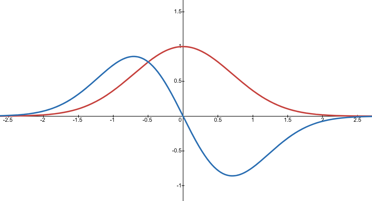
And we see that the force changes sign depending on the position. This yields to a confining potential.
Scattering Force
Let’s get to the second term that we have encountered in the force equation. Once again, let’s just write it down
\[\begin{align*} \mathbf{F}_s &= -\frac{\hbar\mathbf{k}\Omega(\mathbf{r})}{2} \, \frac{\Gamma\Omega/2}{(\Gamma/2)^2 + \delta^2 + \Omega^2/2} \\ &= \hbar\mathbf{k}\Gamma \frac{\Omega^2/4}{(\Gamma/2)^2 + \delta^2 + \Omega^2/2} \end{align*}\]As the ion moves with velocity $\mathbf{v}$, the detuning will change according to the Doppler shift
\[\delta(\mathbf{v}) = \delta - \mathbf{k} \cdot \mathbf{v}\]Therefore, the expression for the scattering force becomes
\[\mathbf{F}_s(\mathbf{v}) = \hbar\mathbf{k}\Gamma \frac{\Omega^2/4}{(\Gamma/2)^2 + (\delta - \mathbf{k}\cdot\mathbf{v})^2 + \Omega^2/2}\]Assuming low velocities, the scattering force as a function of velocity $\mathbf{v}$ becomes
\[\begin{align*} \mathbf{F}_s(\mathbf{v}) &= \mathbf{F}_s(0) + \nabla_\mathbf{v}\mathbf{F}_s(\mathbf{v})\Big\vert_{\mathbf{v} = \mathbf{0}} \cdot \mathbf{v} + o\left(v^2\right) \\ &= \hbar\mathbf{k}\Gamma \frac{\Omega^2/4}{(\Gamma/2)^2 + (\delta - \mathbf{k}\cdot\mathbf{v})^2 + \Omega^2/2} +\hbar\Gamma (\mathbf{k}\cdot\mathbf{v}) \, \nabla_\mathbf{v}\left(\frac{\Omega^2/4}{(\Gamma/2)^2 + (\delta - \mathbf{k}\cdot\mathbf{v})^2 + \Omega^2/2}\right)\Bigg\vert_{\mathbf{v} = 0} \\ &= \hbar\mathbf{k}\Gamma \frac{\Omega^2/4}{(\Gamma/2)^2 + (\delta - \mathbf{k}\cdot\mathbf{v})^2 + \Omega^2/2} +\hbar\mathbf{k}\Gamma \,\frac{\delta\Omega^2/2}{\left((\Gamma/2)^2 + (\delta - \mathbf{k}\cdot\mathbf{v})^2 + \Omega^2/2\right)^2}\,(\mathbf{k}\cdot\mathbf{v}) \\ &= \mathbf{F_0} + \underbrace{\eta v k^2 \cos(\theta)}_{\mathbf{F}_s^{(2)}} \end{align*}\]where we have defined $\mathbf{k}\cdot\mathbf{v} = kv\cos(\theta)$. We are now faced with two terms:
- The first term produces a constant force and needs to be counteracted, for instance with a dipole force term.
- The second one produces a force that is similar to friction.
Let’s see how we get a friction term. To this end, we consider the 1D case and choosing $\theta = \pi$, we get
\[\mathbf{F}_s^{(2)} = \eta k \dot{x}\]which looks like a friction term, thus this is why this force cools down the motion of our atom.