6. Trapped Ions Basics
his set of notes is heavily inspired from Daniel Kienzler’s course on Trapped Ion Physics.
Today we will discuss trapped ions as a quantum computation platform. First, we will see how we can trap an ion into a three-dimensional harmonic oscillator. Then, we will see how we can perform single- and two-qubit gate operations. We will then briefly mention ways of scaling trapped-ion quantum computers.
Trapping an Ion
If we want to work with an ion (or a small ensamble of ions) we first need to trap them. As previously discussed, we will need two fundamental “ingredients”: confinement and cooling.
Given the charge of the ion, it is natural to think of electric fields to create a confining potential. One naive approach would be to have a static electric field of the form
\[\varphi(x,y,z) = \alpha_x x^2 + \alpha_y y^2 + \alpha_z z^2\]However, it turns out that a static electric (or magnetic) cannot confine along all three directions. To see this, we consider Gauss’ theorem for the electric field, namely
\[\nabla \cdot \mathbf{E} = \frac{\rho}{\varepsilon}\]We can then combine it with the definition of the electric field from its potential as $\mathbf{E} = -\nabla\varphi$ to get the following
\[\nabla^2\varphi = -\frac{\rho}{\varepsilon}\]Since we are considering free space, we set $\rho = 0$ and obtain the Laplacian of the electric field potential, namely
\[\frac{\partial^2\varphi}{\partial x^2} + \frac{\partial^2\varphi}{\partial y^2} +\frac{\partial^2\varphi}{\partial y^2} = 0\]From the equation above, we see that for our three-dimensional static harmonic potential, the following equation must be valid
\[\alpha_x + \alpha_y + \alpha_z = 0\]Thus, at least one of the constants must be negative, resulting in one or more directions where the potential is anti-confining.
Paul Trap (Quadrupole Ion Trap)
To get around the limitation that we ran into, we can consider time-varying electric fields. Specifically, let’s consider the electric field potential of the form
\[\varphi(x,y,z,t) = \beta_z z^2 + \beta_r\cos(\Omega t) (x^2 -y^2)\]This is the electric potential that results from the Paul trap geometry, namely 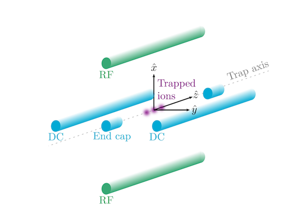
For now, let’s consider $t = 0$. At this time instant, the electric potential is confinin along $z$ and $x$, while anti-confining along $y$. If we now consider $t = \pi/\Omega$, the situation is now flipped. While the potential is still confining along $z$, now we have confinement along $y$ and anti-confinement along $x$. Intuitively, if we swap the confinement and anticonfinement directions quickly enoung ($\Omega$ is high enough), then we would be able to confine the charged particle. In fact, any unwanted anti-confinement would be quickly rectified by confinement.
In particular, in the field described above we have two components: a static (DC) harmonic potential along the $z$ (axial) direction and a time-varying (RF) quadrupole field in the $x$ and $y$ (radial) directions. It can be proven that, under certain assumptions, the result is a quasi-harmonic potential in all three directions. In particular, the time evolution for the particle radial position $u = {x,y}$ is given by
\[u(t) = A \underbrace{\cos(\omega_\text{sec}t)}_\text{secular motion}\underbrace{\left(1-\frac{q_u}{2}\cos(\Omega t)\right)}_\text{micro-motion}\]where both $\omega_\text{sec}$ and $q_u$ depend on the trapping parameters. We see two distinct components of the particle’s motion:
- micromotion: induced by the time-variations of the electric field
- secular motion results from the time averaging of the effects of the changing field. It can be described as being caused by a perfect harmonic potential
Loading into a Trap
We now have our three-dimensional confining potential. The first thing we want to do is to load an ion in it. While there are many ways of doing this, the most common is by boiling off neutral atoms from an oven. Lasers are then used to excite the outermost electron to the continuum. Consider neutral calcium:
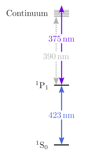
Image reproduced from R. Oswald, Characterization and control of a cryogenic ion trap apparatus and laser systems for quantum computing
With two lasers, one at $423\,\text{nm}$ and one at $375 \,\text{nm}$, we can ionise an atom of calcium to $\text{Ca}^+$. We can then use laser cooling to slow down the ion and eventually loading it into the Paul trap that we described above.
Performing Operations on the Ion
Now that we have trapped an ion and cooled its motion to a satisfactory level, we want to work with it. In particular we will need to
- Initialise its state
- Perform single- and multi-qubit gate operations
- Readout its state
To this end, we need to chose which levels we want to work with. Once again, let’s go back to the energy level diagram for $\text{Ca}^+$:
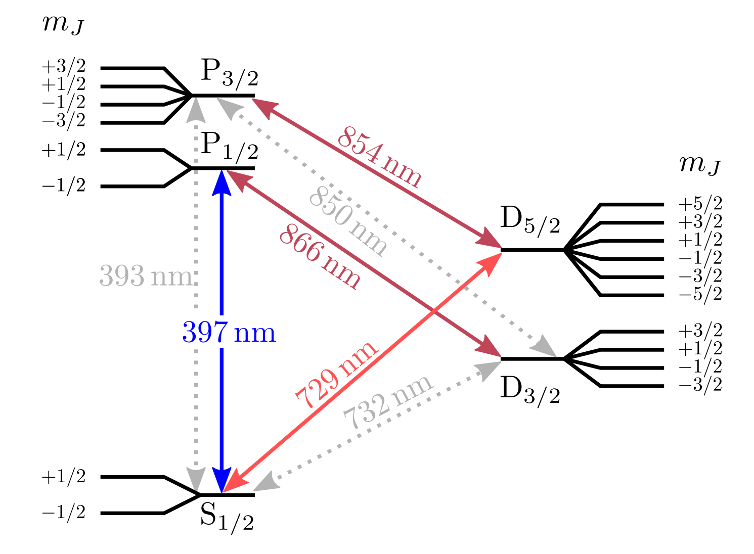
Image reproduced from R. Oswald, Characterization and control of a cryogenic ion trap apparatus and laser systems for quantum computing
We will encode our qubit between the $S_{1/2}$ and $D_{5/2}$ levels. This is because this is a dipole-forbidden transition and as a result, it does not decay easily. This is crucial to bump up the $T_1$ spin coherence of our qubit.
Readout
While this is ideal to store quantum information, the same cannot be said about reading it out. In fact, we would have to wait for a long time before we can readout our qubit.
To solve this issue, we can perform the qubit readout with the help of a second transition: $S_{1/2}\leftrightarrow P_{1/2}$. This time, this transition is dipole-allowed and therefore decays rather quickly. This allows us to perform state-dependent fluorescence readout of our ion’s state. If the spin is in the $S_{1/2}$ manifold, the ion would be bright under $397\,\text{nm}$ light. Instead, if the spin is in the $D_{5/2}$ manifold, no fluorescence occurs.
We should note that, once excited to the $P_{1/2}$ level, the ion has a small chance of decaying into the $D_{3/2}$ manifold. For this reason, it is importnat to repump out of it back into the $P_{1/2}$ manifold. To this end we add a repumper laser at $732\,\text{nm}$
State Preparation
Another operation that is crucial for the operation of a quantum information processing system is state preparation. We need some sort of non-unitary process whose dark state is the state we want to achieve. In particular, we need to select a particular level within the fine structure of the $S_{1/2}$ ground state manifold.
We can use two different ways of doing that 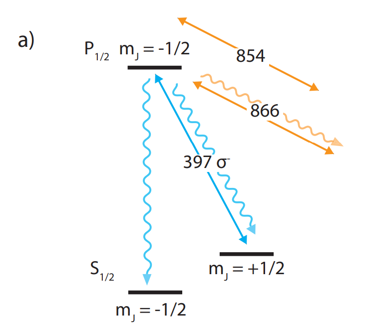
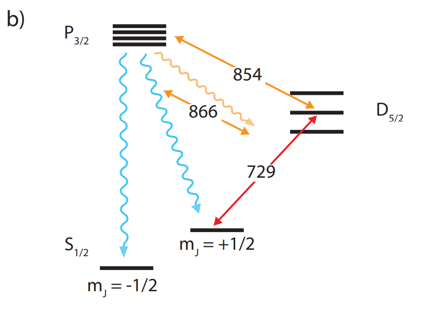
Image reproduced from M. Malinowski, Unitary and Dissipative Trapped-Ion Entanglement Using Integrated Optics
Either we use $\sigma$-polarised $397\,\text{nm}$ light (alighne) to exploit the dipole selection rules or we can use the narrow $729\,\text{nm}$ light to repump out of the wrong sublevel.
Spin-Motion Coupling
To perform computation, we need to apply single- and multi-qubit gates. In both cases, we rely on the following Hamiltonian:
\[\hat{H} = \frac{\hbar\Omega}{2}\hat{\sigma}_+\left[\mathbb{I} + i\eta\left(\hat{a}e^{-it(\delta + \omega_x)} + \hat{a}^\dagger e^{-it(\delta - \omega_x)}\right)\right]+\text{h.c.}.\]In particular, we see three main terms. We will see that one term allows us to drive Rabi flops between the $\vert g\rangle$ and $\vert e\rangle$ states, while the other two terms will allow us to exchange excitations between the motional and the motion degree of freedom.
The result is that, by tuning the frequency of the laser, one can choose which terms of the Hamiltonian to apply and which to suppress. In turn, this allows us to trasverse the state ladder composed of the spin and motional degrees of freedom.
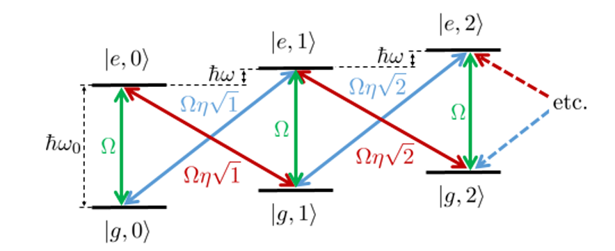
This is extremely useful to ground-state cool and to perform multi-qubit gates. In the former case, we drive “Red-sidebands” together with optical repumping to climb down the ladder.