8. On the Quest of Making Artificial Atoms
We are on a quest to create an “artificial atom”. By that, we mean a system that has some key characteristics of an atom. To be precise, we look for
- Two levels that only interact with eachother. This is where we will encode our qubit
- A way of manipulating the state of the qubit
- A way of reading out the state of the qubit
- Long coherence times
A potential place to look is the quantum harmnonic oscillator. In the case of superconducting qubits, the harmonic oscillator we consider is of the LC circuit.
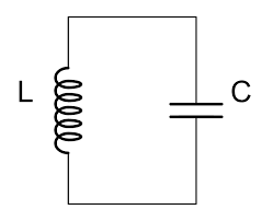
We know that the total energy in the system is given by
\[H = \frac{1}{2}LI^2 + \frac{1}{2}CV^2\]However, we know that $\Phi = LI$, and $V=L\dot{I}=\dot{\Phi}$. Substituting in the equation above, we get
\[H = \frac{C}{2}\dot{\Phi}^2 + \frac{1}{2L}\Phi^2\]We clearly see the resemblance to the mechanical harmonic oscillator, where the Hamiltonian is given by
\[H = \frac{1}{2}m\dot{x}^2 + \frac{1}{2}m\omega^2x^2\]Similarly to the mechanical oscillator, we can quantise the LC harmonic oscillator. To this end, we postulate that charge $Q = CV = C\dot{\Phi}$ and flux $\Phi$ are operators and have the following commutation relation
\[\left[\hat{\Phi}, \hat{Q}\right] = i\hbar\mathbb{I}\]We can pull the usual tricks and end up in the Fock picture. In particular, we get equally spaced energy levels
\[E_n = \left(\frac{1}{2} + n\right)\hbar\omega, \ \omega=\frac{1}{\sqrt{LC}}\]Let’s now try to encode our qubit. We might naively use the $\vert 0\rangle$ and $\vert 1\rangle$ states. Then we could consider $\hat{a}$ and $\hat{a}^\dagger$ as our $\hat{\sigma}_{-}$ and $\hat{\sigma}_{+}$ operators respectively. The issue is that, in this way, not only we can couple $\vert 0\rangle \leftrightarrow \vert 1\rangle$, we will also couple the higher fock states $\vert 1\rangle \leftrightarrow \vert 2\rangle, \vert 2\rangle \leftrightarrow \vert 3\rangle,\dots$ and this is boviously not wanted. To solve this issue, we could try to introduce some uneven spacing of the energy levels. In other words, we need to introduce anharmonicity (or non-linearity) in our harmonic oscillator.
The Josephson Junction
The standard way of introducting this non-linearity in superconducting circuits is to use Josephson junctions. This particular type of junction is made of two superconducting electrodes separated by a small insulator.
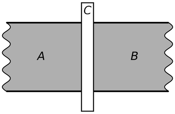
The typical circuit diagram for the Josephson junction is given by a wire with a cross on top. It turns out that, the Josephson junction behaves like an inductor, although with a significant difference. Let’s write the josephson equations
\[\begin{align*} I(t) &= I_c \sin\varphi(t) \\ \frac{\partial\varphi}{\partial t} &= \frac{2eV(t)}{\hbar} \end{align*}\]We see that the sine term in $I = I_c \sin \phi$ is nonlinear. Linear systems would have $I \propto \phi$, but here the relationship is sinusoidal. This gives us the source of non-linearity that we needed.
Cavity Coupling
To readout our qubit, we can dispersively couple it to a cavity (in the MW regime). The interaction hamiltonian that results from this interaction would be of the form
\[\hat{H}_I \approx \hbar\chi\hat{a}^\dagger\hat{a}\hat{\sigma}_z\]where $\hat{\sigma}_z$ acts on our qubit. We see that the cavity energies are shifted around by the state of our qubit. Therefore, by probin the cavity that is coupled to the qubit, we can readout the state of our two-level system.