9. Superconductiong Qubits
In this section, we will explore the Josephson Junction in greater detail. First, we will derive the Josephson equations, that we mentioned in the previous section. Then, we will derive the dispersive interaction between a two level system and a cavity mode. This, as we will see, will allow us to readout the state of the supercondicting qubit.
Josphson Equations
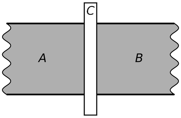
The Josephson unction is made of two superconducting electrodes separated by a small insulator, as shown in the figure below.
By symmetry, we can assume that the wavefunction is constant across the two regions, thus we can write the total wafefunction as
\[\vert\Psi\rangle = \begin{bmatrix} \Psi_1 \\ \Psi_2 \end{bmatrix}\]where $\Psi_1$ and $\Psi_2$ are the wafefunctions in region one and two respectively. Since we apply a voltage to the two conductors, we will induce a splitting of the energies. We can describe this with the Hamiltonian
\[\hat{H}_s = \begin{bmatrix} \frac{qV}{2} && 0 \\ 0 && -\frac{qV}{2} \end{bmatrix}\]Where $q=2e$ is the charge of one Cooper pair (composed of two electrons). In addition, since we have a thin insulator between the two superconductors, we will have some tunnelling at rate $K$. This will induce coupling between the two wavefunctions, and can be described with
\[\hat{H}_i = \begin{bmatrix} 0 && K \\ K && 0 \end{bmatrix}\]Putting it all together, we get that the total hamiltonian $\hat{H} = \hat{H}_s + \hat{H}_i$ is given by
\[\hat{H} = \begin{bmatrix} \frac{qV}{2} && K \\ K && -\frac{qV}{2} \end{bmatrix}\]Giving us the Schrödinger equation
\[i\hbar\frac{\mathrm{d}}{\mathrm{d}t}\vert\Psi\rangle = \hat{H}\vert\Psi\rangle\]In reality, we will not be dealing with single Cooper pairs, but with macroscopic quantities that arise from large ensambles of $N$ Cooper pairs. To better describe this scenario, we divide both sides of the Schrödinger equation by $\sqrt{qN}$, to get
\[i\hbar\frac{\mathrm{d}}{\mathrm{d}t}\vert\psi\rangle = \hat{H}\vert\psi\rangle\]With $\vert\psi\rangle = \sqrt{qN}\,\vert\Psi\rangle$. The nice thing about $\vert\psi\rangle$ is that it is closely connected with the macroscopic charge of the system as
\[Q = \iiint_V |\psi(x,y,z)|^2 \mathrm{d}V\]To proceed, we write the differential equations we get out of the Schrödinger equation
\[\begin{cases} i\hbar\dot{\psi}_1 = +\frac{qV}{2}\psi_1 + K\psi_2 \\ i\hbar\dot{\psi}_2 = -\frac{qV}{2}\psi_2 + K\psi_1 \end{cases}\]We can then parametrise $\psi_j = \sqrt{\rho_j}e^{i\theta_j}$, where $\rho_j$ and $\theta_j$ are the charge density and phase respectively. As we substitute and do some algebra, we end up with
\[\begin{cases} \dot{\theta}_2 - \dot{\theta}_1 = \frac{qV}{\hbar} + \frac{K}{\hbar}\left(\sqrt\frac{\rho_2}{\rho_1} - \sqrt\frac{\rho_1}{\rho_2}\,\right) \cos(\theta_2 - \theta_1) \\ \dot{\rho}_1 = \frac{2K\sqrt{\rho_1\rho_2}}{\hbar}\sin(\theta_2 - \theta_1) \end{cases}\]To simplify things, we introduce the relative phase $\varphi = \theta_2 - \theta_1$ and we assume that the charge density is almost the same across the junction, namely $\rho_1 \approx \rho_2 = \rho_0$. We also note that $\dot{\rho}_0$ is equivalent to the current density $J$ across the junction. Therefore we get
\[\begin{align*} \dot{\varphi} &= \frac{qV}{\hbar} \\ J &= J_0 \sin\varphi \end{align*}\]where $J_0 = 2K\rho_0/\hbar$. We can integrate over the junction surface, since
\[I = \iint_S \mathbf{J}\cdot\mathrm{d}\mathbf{S}\]Thus, we get the final form of the Josephson equations
\[\begin{align*} V &= \frac{\Phi_0}{2\pi}\dot{\varphi} \\ I &= I_c\sin\varphi \end{align*}\]where $\Phi_0 = \hbar/2e$ is the quantum flux and $I_c$ is the critical current of the junction.
Josephson Junction as a Non-Linear Element
We can now assume steady state, and expand the second equation. To this end, we will introduce the effective magnetic flux $\tilde{\Phi}=\Phi_0\frac{\varphi}{2\pi}$. The current equation then becomes
\[I = I_c \sin\left(\frac{2\pi\tilde{\Phi}}{\Phi_0}\right) = I_c\frac{2\pi\tilde{\Phi}}{\Phi_0} - \frac{I_c}{3!}\left(\frac{2\pi\tilde{\Phi}}{\Phi_0}\right)^3 + \mathcal{o}\left(\tilde{\Phi}^5\right)\]We can compare it with an inductor, whose relationship is
\[L = \frac{\Phi}{I}\]Thus the Josephson junction behaves as an inductor having inductance
\[L_J = \frac{\Phi_0}{2\pi I_c}\]And most importantly, it shows a non-linear behaviour, that can be seen from the second term. Terefore, we can “substitute” our normal inductor in the LC circuit with a Josephson junction to get the anharmonicity we desire.
Cavity-Qubit Interaction: Dispersive Hamiltonian
This section of the notes is inspired from Atac Imamoglu’s course on Quantum Optics.
We now discuss how we can readout the state of a superconducting qubit with the help of a cavity mode. To this end, we write the Hamiltonian for the system composed of a single qubit interacting with a cavity mode:
\[\hat{H} = \underbrace{\frac{\hbar\omega_{eg}}{2}\hat{\sigma}_z}_\text{qubit energy} + \underbrace{\hbar\omega_c\hat{a}^\dagger\hat{a}}_\text{cavity energy} + \hbar g_c\left(\hat{\sigma}_+\hat{a} + \hat{a}^\dagger\hat{\sigma}_+\right)\]We want to consider the limit where $\vert\omega_{eg} - \omega_c\vert \gg g_c$, the so-called dispersive limit. To this end, we divide the Hamiltonian into $\hat{H}_0$ and $\hat{H}_1$ as
\[\hat{H} = \hat{H}_0 + \hat{H}_1\]Where
\[\begin{align*} \hat{H}_0 &= \frac{\hbar\omega_{eg}}{2}\hat{\sigma}_z + \hbar\omega_c\hat{a}^\dagger\hat{a} \\ \hat{H}_1 &= \hbar g_c\left(\hat{\sigma}_+\hat{a} + \hat{a}^\dagger\hat{\sigma}_+\right) \end{align*}\]Note that $\hat{H}0$ has know eigenstates ${\vert i\rangle \otimes \vert n \rangle}$ with $i = 1,2$ and $n = 1,2,3,\dots$ We also notice that $\hat{H}_1$ is completely off-diagonal. The goal is to write down the Hamiltonian in such a way that we can see what dynamics we can disregard considering $\vert\omega{eg} - \omega_c\vert \gg g_c$. To this end, we introduce the general unitary transformation
\[\hat{H} \to e^{-\hat{S}}\hat{H}e^{\hat{S}}\]We are now left with the task of chosing $\hat{S}$. This is part of the Schrieffer-Wolff transformation. We now introduce $\Delta\omega = \omega_{eg}-\omega_c$ and apply Baker–Campbell–Hausdorff formula to get
\[\begin{align*} \hat{H} \to e^{-\hat{S}}\hat{H}e^{\hat{S}} &= \hat{H} + [\hat{S}, \hat{H}] + \frac{1}{2}[\hat{S}, [\hat{S}, \hat{H}]] + \dots \\ &= \hat{H}_0 + \hat{H}_1 + [\hat{S}, \hat{H}_0] + [\hat{S}, \hat{H}_1] + \frac{1}{2}[\hat{S}, [\hat{S}, \hat{H}_0]] +\frac{1}{2}[\hat{S}, [\hat{S}, \hat{H}_1]] + \dots \end{align*}\]A sensible choice of $\hat{S}$ is such that
\[\left[\hat{S}, \hat{H}_0\right] = -\hat{H}_1\]Since this will reduce the expression above to
\[\begin{align} \hat{H} \to e^{-\hat{S}}\hat{H}e^{\hat{S}} &= \hat{H}_0 + [\hat{S}, \hat{H}_1] - \frac{1}{2}[\hat{S}, \hat{H}_1] +\frac{1}{2}[\hat{S}, [\hat{S}, \hat{H}_1]] + \dots \\ &= \hat{H}_0 + \frac{1}{2}[\hat{S}, \hat{H}_1] + O(\hat{V}^3) \end{align}\]The interesting thing is that, both $\hat{H}_0$ and $\frac{1}{2}[\hat{S}, \hat{H}_1]$ are diagonal Hamiltonians. Thus, if we truncate to the first order, we can obtain a diagonal expression for the Hamiltonian.
In our case, the choice for $\hat{S}$ is
\[\hat{S} = \frac{g_c}{\Delta\omega}\left(\hat{\sigma}_+\hat{a} - \hat{a}^\dagger\hat{\sigma}_+\right)\]Note that singe $g_c \ll \Delta\omega$, we can comfortably truncate to the first term. This leaves us with
\[\begin{align*} \hat{H} &\approx \overbrace{\frac{\hbar\omega_{eg}}{2}\hat{\sigma}_z + \hbar\omega_c\hat{a}^\dagger\hat{a}}^{\hat{H}_0} + \frac{\hbar g_c^2}{2\Delta\omega}\left[\hat{\sigma}_+\hat{a} + \hat{a}^\dagger\hat{\sigma}_+, \hat{\sigma}_+\hat{a} - \hat{a}^\dagger\hat{\sigma}_+\right] \\ &= \frac{\hbar\omega_{eg}}{2}\hat{\sigma}_z + \hbar\omega_c\hat{a}^\dagger\hat{a} + \frac{\hbar g_c^2}{2\Delta\omega^2}\hat{\sigma}_z + \frac{\hbar g_c^2}{\Delta\omega}\hat{a}^\dagger\hat{a}\hat{\sigma}_z \end{align*}\]Let us analyse what we have. The term $\frac{\hbar g_c^2}{2\Delta\omega^2}\hat{\sigma}_z$ is a stark shiftt induced by the detuning of the cavity with respect to the qubit. More interestingly, the term $\frac{\hbar g_c^2}{\Delta\omega}\hat{a}^\dagger\hat{a}\hat{\sigma}_z$ allows for the dispersive interaction. We note that the energy spacing of the cavity mode is modified depending on the state of the qubit, via the $\hat\sigma_z$ term. In this way, we can readout the state of the qubit by looking at the cavity resonance.